NetworkLayout
This is the Documentation for NetworkLayout.
All example images on this page are created using Makie.jl and the graphplot recipe from GraphMakie.jl.
using CairoMakie
using NetworkLayout
using GraphMakie, Graphs
Basic Usage & Algorithms
All of the algorithms follow the Layout Interface. Each layout algorithm is represented by a type LayoutAlgorithm <: AbstractLayout. The parameters of each layout can be set with keyword arguments. The LayoutAlgorithm object itself is callable and transforms the adjacency matrix and returns a list of Point{N,T} from GeometryBasics.jl.
alg = LayoutAlgorithm(; p1="foo", p2=:bar)
positions = alg(adj_matrix)
Each of the layouts comes with a lowercase function version:
positions = layoutalgorithm(adj_matrix; p1="foo", b2=:bar)Instead of using the adjacency matrix you can use AbstractGraph types from Graphs.jl directly.
g = complete_graph(10)
positions = layoutalgorithm(g)
Scalable Force Directed Placement
NetworkLayout.SFDP — Type
SFDP(; kwargs...)(adj_matrix)
sfdp(adj_matrix; kwargs...)
Using the Spring-Electric model suggested by Hu (2005, The Mathematica Journal, pdf).
Forces are calculated as:
    f_attr(i,j) = ‖xi - xj‖ ² / K ,    i<->j
    f_repln(i,j) = -CK² / ‖xi - xj‖ ,  i!=j
Takes adjacency matrix representation of a network and returns coordinates of the nodes.
Keyword Arguments
dim=2,Ptype=Float64: Determines dimension and output typePoint{dim,Ptype}.tol=1.0: Stop if position changes of last stepΔp <= tol*Kfor all nodesC=0.2,K=1.0: Parameters to tweak forces.iterations=100: maximum number of iterationsinitialpos=Point{dim,Ptype}[]Provide
VectororDictof initial positions. All positions will be initialized using random coordinates between [-1,1]. Random positions will be overwritten using the key-val-pairs provided by this argument.pin=[]: Pin node positions (won't be updated). Can be given asVectororDictof node index -> value pairings. Values can be either(12, 4.0): overwrite initial position and pintrue/false: pin this position(true, false, false): only pin certain coordinates
seed=1: Seed for random initial positions.rng=DEFAULT_RNG[](seed)Create rng based on seed. Defaults to
MersenneTwister, can be specified by overwritingDEFAULT_RNG[]
Example
g = wheel_graph(10)
layout = SFDP(Ptype=Float32, tol=0.01, C=0.2, K=1)
f, ax, p = graphplot(g, layout=layout)
hidedecorations!(ax); hidespines!(ax); ax.aspect = DataAspect(); f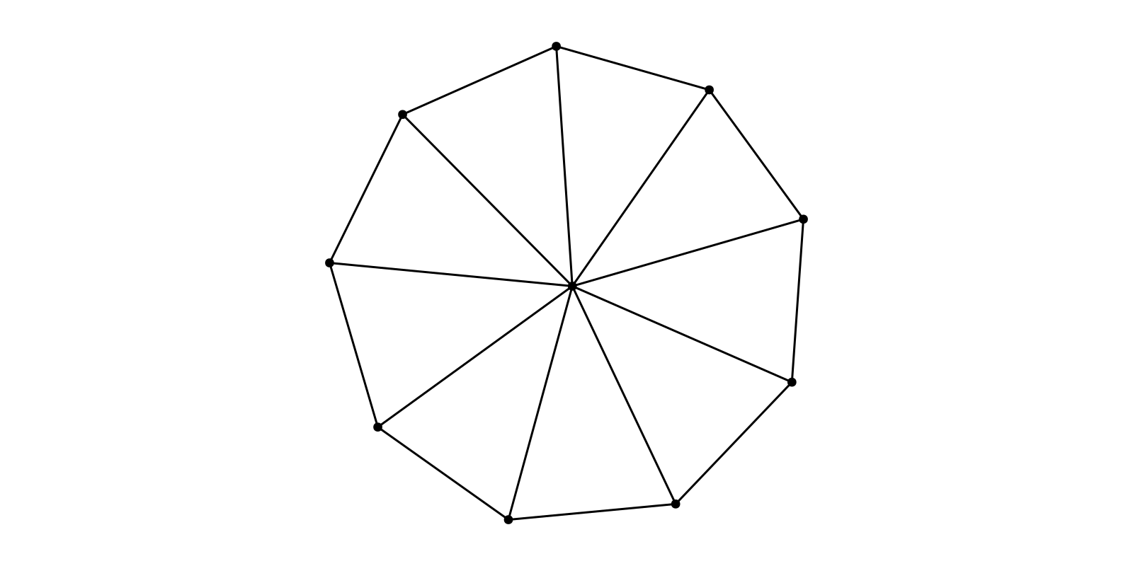
Iterator Example
iterator = LayoutIterator(layout, g)
record(f, "sfdp_animation.mp4", iterator; framerate = 10) do pos
    p[:node_pos][] = pos
    autolimits!(ax)
endBuchheim Tree Drawing
NetworkLayout.Buchheim — Type
Buchheim(; kwargs...)(adj_matrix)
Buchheim(; kwargs...)(adj_list)
buchheim(adj_matrix; kwargs...)
buchheim(adj_list; kwargs...)
Using the algorithm proposed by Buchheim, Junger and Leipert (2002, doi 10.1007/3-540-36151-0_32).
Takes adjacency matrix or list representation of given tree and returns coordinates of the nodes.
Keyword Arguments
Ptype=Float64: Determines the output typePoint{2,Ptype}.nodesize=Float64[]Determines the size of each of the node. If network size does not match the length of
nodesizefill up withonesor truncate given parameter.
Example
adj_matrix = [0 1 1 0 0 0 0 0 0 0;
              0 0 0 0 1 1 0 0 0 0;
              0 0 0 1 0 0 1 0 1 0;
              0 0 0 0 0 0 0 0 0 0;
              0 0 0 0 0 0 0 1 0 1;
              0 0 0 0 0 0 0 0 0 0;
              0 0 0 0 0 0 0 0 0 0;
              0 0 0 0 0 0 0 0 0 0;
              0 0 0 0 0 0 0 0 0 0;
              0 0 0 0 0 0 0 0 0 0]
g = SimpleDiGraph(adj_matrix)
layout = Buchheim()
f, ax, p = graphplot(g, layout=layout)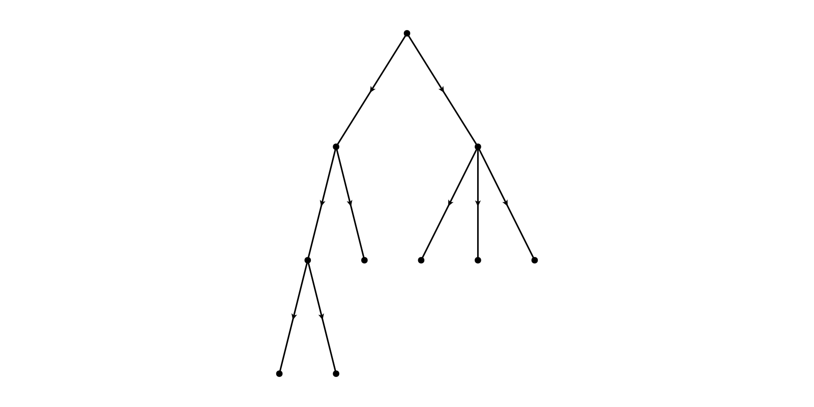
Spring/Repulsion Model
NetworkLayout.Spring — Type
Spring(; kwargs...)(adj_matrix)
spring(adj_matrix; kwargs...)
Use the spring/repulsion model of Fruchterman and Reingold (1991, doi 10.1002/spe.4380211102) with
- Attractive force:
f_a(d) = d^2 / k - Repulsive force:
f_r(d) = -k^2 / d
where d is distance between two vertices and the optimal distance between vertices k is defined as C * sqrt( area / num_vertices ) where C is a parameter we can adjust
Takes adjacency matrix representation of a network and returns coordinates of the nodes.
Keyword Arguments
dim=2,Ptype=Float64: Determines dimension and output typePoint{dim,Ptype}.C=2.0: Constant to fiddle with density of resulting layoutiterations=100: maximum number of iterationsinitialtemp=2.0: Initial "temperature", controls movement per iterationinitialpos=Point{dim,Ptype}[]Provide
VectororDictof initial positions. All positions will be initialized using random coordinates between [-1,1]. Random positions will be overwritten using the key-val-pairs provided by this argument.pin=[]: Pin node positions (won't be updated). Can be given asVectororDictof node index -> value pairings. Values can be either(12, 4.0): overwrite initial position and pintrue/false: pin this position(true, false, false): only pin certain coordinates
seed=1: Seed for random initial positions.rng=DEFAULT_RNG[](seed)Create rng based on seed. Defaults to
MersenneTwister, can be specified by overwritingDEFAULT_RNG[]
Example
g = smallgraph(:cubical)
layout = Spring(Ptype=Float32)
f, ax, p = graphplot(g, layout=layout)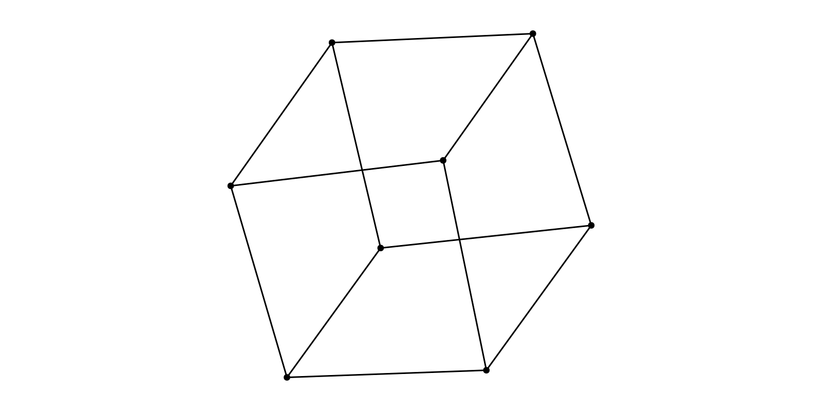
Iterator Example
iterator = LayoutIterator(layout, g)
record(f, "spring_animation.mp4", iterator; framerate = 10) do pos
    p[:node_pos][] = pos
    autolimits!(ax)
endAligning Layouts
Any two-dimensional layout can have its principal axis aligned along a desired angle (default, zero angle), by nesting an "inner" layout into an Align layout. For example, we may align the above Spring layout of the small cubical graph along the horizontal or vertical axes:
NetworkLayout.Align — Type
Align(inner_layout :: AbstractLayout{2, Ptype}, angle :: Ptype = zero(Ptype))Align the vertex positions of inner_layout so that the principal axis of the resulting layout makes an angle with the x-axis. Also automatically centers the layout origin to its center of mass (average node position).
Only supports two-dimensional inner layouts.
g = smallgraph(:cubical)
f, ax, p = graphplot(g, layout=Align(Spring())) # horizontal alignment (zero angle by default)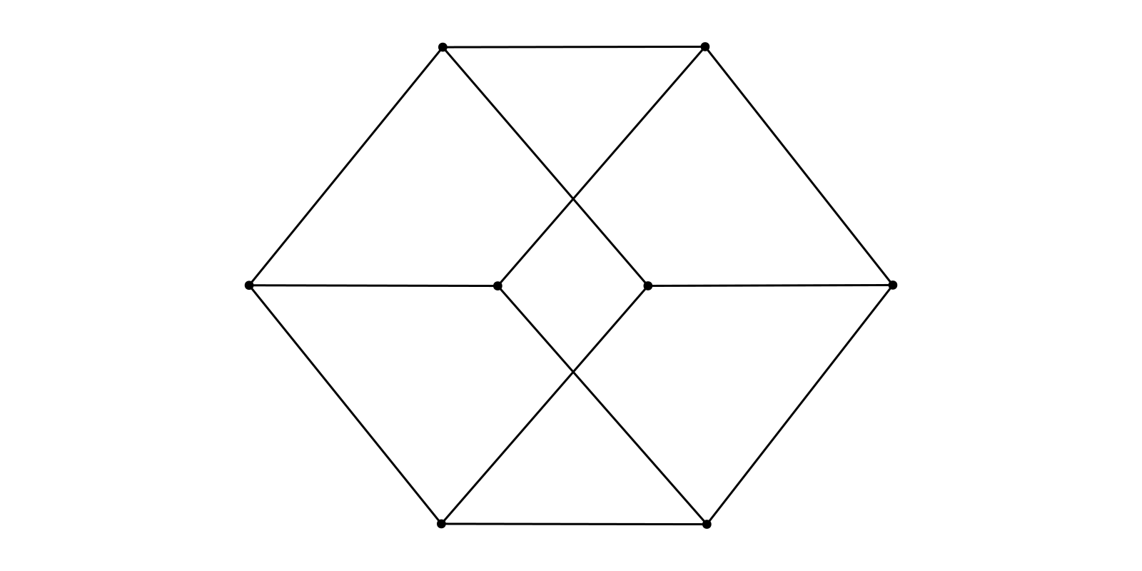
f, ax, p = graphplot(g, layout=Align(Spring(), pi/2)) # vertical alignment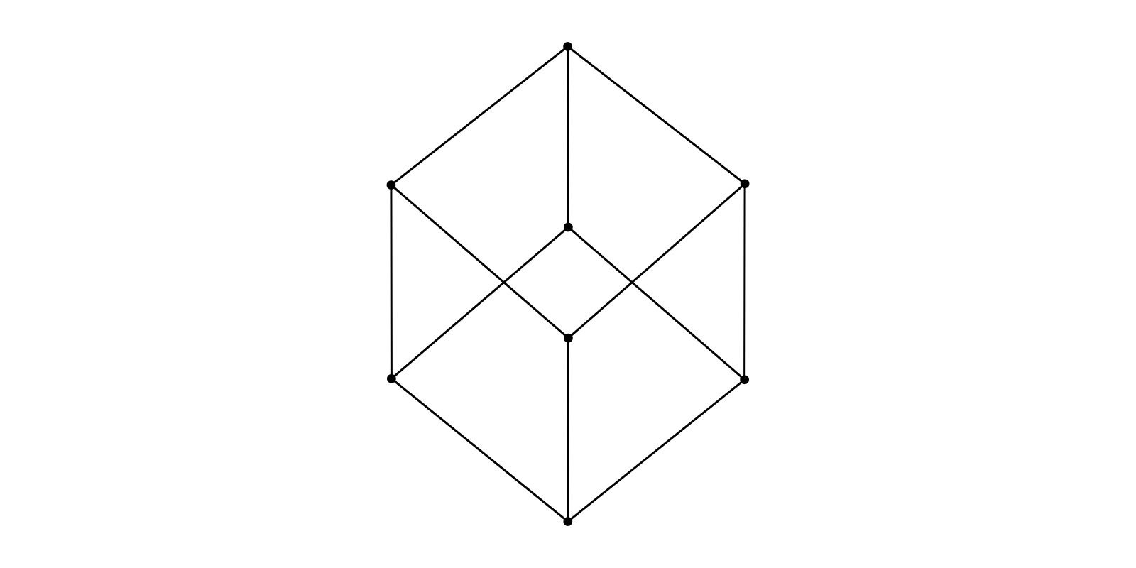
Stress Majorization
NetworkLayout.Stress — Type
Stress(; kwargs...)(adj_matrix)
stress(adj_matrix; kwargs...)
Compute graph layout using stress majorization. Takes adjacency matrix representation of a network and returns coordinates of the nodes.
The main equation to solve is (8) in Gansner, Koren and North (2005, doi 10.1007/978-3-540-31843-9_25).
Inputs:
adj_matrix: Matrix of pairwise distances.
Keyword Arguments
dim=2,Ptype=Float64: Determines dimension and output typePoint{dim,Ptype}.iterations=:auto: maximum number of iterations (:automeans400*N^2whereNare the number of vertices)abstols=0Absolute tolerance for convergence of stress. The iterations terminate if the difference between two successive stresses is less than abstol.
reltols=10e-6Relative tolerance for convergence of stress. The iterations terminate if the difference between two successive stresses relative to the current stress is less than reltol.
abstolx=10e-6Absolute tolerance for convergence of layout. The iterations terminate if the Frobenius norm of two successive layouts is less than abstolx.
weights=Array{Float64}(undef, 0, 0)Matrix of weights. If empty (i.e. not specified), defaults to
weights[i,j] = δ[i,j]^-2ifδ[i,j]is nonzero, or0otherwise.initialpos=Point{dim,Ptype}[]Provide
VectororDictof initial positions. All positions will be initialized using random coordinates from normal distribution. Random positions will be overwritten using the key-val-pairs provided by this argument.pin=[]: Pin node positions (won't be updated). Can be given asVectororDictof node index -> value pairings. Values can be either(12, 4.0): overwrite initial position and pintrue/false: pin this position(true, false, false): only pin certain coordinates
seed=1: Seed for random initial positions.rng=DEFAULT_RNG[](seed)Create rng based on seed. Defaults to
MersenneTwister, can be specified by overwritingDEFAULT_RNG[]uncon_dist=(maxdist, Ncomps)->maxdist*Ncomps^(1/3)Per default, unconnected vertices in the graph get a pairwise "ideal" distance which scales with the number of connected components and the maximum distance within the components.
Example
g = SimpleGraph(936)
for l in eachline(joinpath(@__DIR__,"..","..","test","jagmesh1.mtx"))
    s = split(l, " ")
    src, dst = parse(Int, s[1]), parse(Int, s[2])
    src != dst && add_edge!(g, src, dst)
end

layout = Stress(Ptype=Float32)
f, ax, p = graphplot(g; layout=layout, node_size=3, edge_width=1)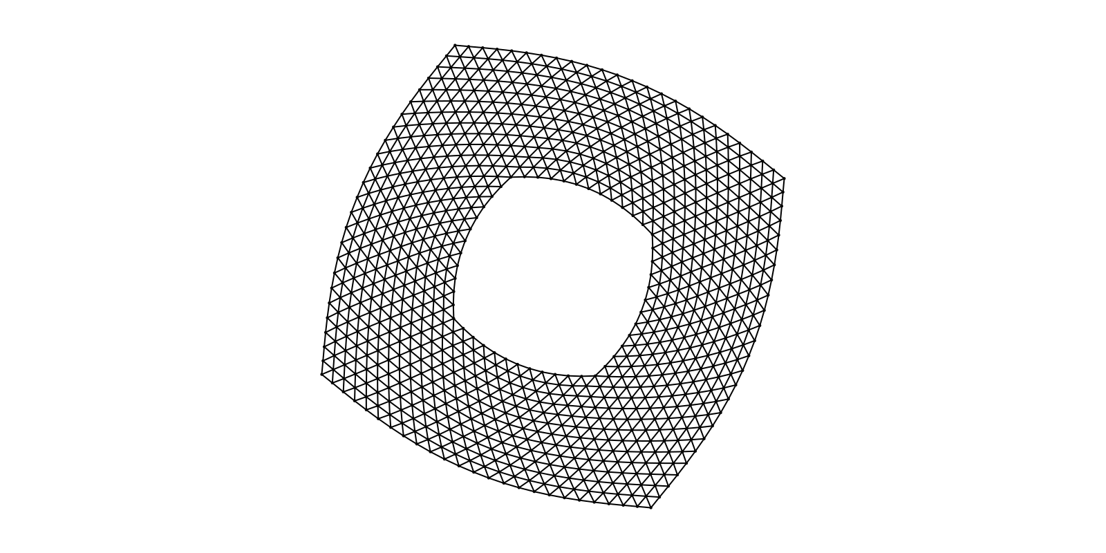
Iterator Example
iterator = LayoutIterator(layout, g)
record(f, "stress_animation.mp4", iterator; framerate = 7) do pos
    p[:node_pos][] = pos
    autolimits!(ax)
endEgocentric Layout
NetworkLayout.Egocentric — Type
Egocentric(; kwargs...)(adj_matrix)
egocentric(adj_matrix; kwargs...)
Compute an egocentric ("focus") graph layout using stress majorization, centered on a single focal vertex. Takes an adjacency matrix representation of a network and returns coordinates of the nodes, translated such that the focal vertex sits at the origin.
The layout interpolates between two objectives, following Brandes and Pich, "More Flexible Radial Layout", Journal of Graph Algorithms and Applications 15(1):157-173 (2011, doi 10.7155/jgaa.00221):
- a plain stress objective, which tries to match all pairwise euclidean distances to the corresponding graph distances (this is
Stress), and - a focus objective, which only weights the pairs involving the focal vertex.
Minimizing the focus objective alone places every vertex at a radius equal to its graph distance from the focal vertex, producing concentric rings of constant geodesic distance. Optimization proceeds along a schedule tseq of mixing parameters t ∈ [0,1], where the weights used in iteration stage t are (1-t)*W + t*Z with W[i,j] = d[i,j]^-2 and Z equal to W on the row and column of the focal vertex and zero elsewhere. Each stage is majorized to convergence before moving on to the next. Starting at t=0 and ending at t=1 therefore uses the unconstrained stress layout to pick sensible angles, then gradually enforces the radii.
Inputs:
adj_matrix: Matrix of pairwise distances.
Keyword Arguments
focus=1: Index of the focal vertex. It is held at the origin, so all returned positions are relative to it. Pinning it has no effect.dim=2,Ptype=Float64: Determines dimension and output typePoint{dim,Ptype}.tseq=0.0:0.1:1.0Schedule of mixing parameters, from pure stress (
t=0) to pure focus (t=1). Must be non-empty with entries in[0,1].iterations=100: maximum number of majorization steps per entry oftseq.abstols=0.0Absolute tolerance for convergence of stress. A stage terminates if the difference between two successive stresses is less than abstol.
reltols=10e-5Relative tolerance for convergence of stress. A stage terminates if the improvement in stress relative to the current stress is less than reltol.
abstolx=10e-6Absolute tolerance for convergence of layout. A stage terminates if the largest movement of any single node is less than abstolx.
maxdist=nothingIf given, radially compress every vertex further than
maxdistfrom the focal vertex onto a narrow band outsidemaxdist, keeping its angle. This bounds the extent of the layout so that the interesting, near part of the network fills the frame. Vertices that are unconnected to the focal vertex are affected by this too (seeuncon_dist). Withoutmaxdistno compression is applied.compress=log1pHow far past
maxdista vertex at excess radiusΔ = r - maxdistis drawn: its new radius ismaxdist + compress(Δ). May be a function, a real number (all distant vertices land on a single ring atmaxdist + compress), ornothing(equivalent to0, i.e. clamp onto themaxdistring). Ignored whenmaxdistisnothing.uncon_dist=(maxdist, Ncomps)->maxdist*Ncomps^(1/3)Per default, unconnected vertices in the graph get a pairwise "ideal" distance which scales with the number of connected components and the maximum distance within the components.
initialpos=Point{dim,Ptype}[]Provide
VectororDictof initial positions. By default all positions are initialized using classical multidimensional scaling of the graph distances plus a small random jitter, which makes the result largely deterministic. Those positions will be overwritten using the key-val-pairs provided by this argument.pin=[]: Pin node positions (won't be updated). Can be given asVectororDictof node index -> value pairings. Values can be either(12, 4.0): overwrite initial position and pintrue/false: pin this position(true, false, false): only pin certain coordinates
Pinned positions are given relative to the focal vertex (which sits at the origin), and are exempt from the
maxdistcompression.seed=1: Seed for the random jitter on the initial positions.rng=DEFAULT_RNG[](seed)Create rng based on seed. Defaults to
MersenneTwister, can be specified by overwritingDEFAULT_RNG[]
Example
An egocentric layout puts one vertex at the centre and arranges everyone else on concentric rings, one per geodesic step away from it. The angles still come from a regular stress layout, so vertices that are close in the network stay close on their ring.
g = watts_strogatz(120, 4, 0.3; seed=2)
focus = 1
layout = Egocentric(; focus)

node_color = [i == focus ? :tomato : :black for i in 1:nv(g)]
node_size = [i == focus ? 20 : 6 for i in 1:nv(g)]
f, ax, p = graphplot(g; layout, node_color, node_size, edge_width=0.5)
for r in 1:maximum(gdistances(g, focus))
    arc!(ax, Point2f(0), r, -pi, pi; color=(:gray, 0.5), linewidth=0.5)
end
hidedecorations!(ax); hidespines!(ax); ax.aspect = DataAspect(); f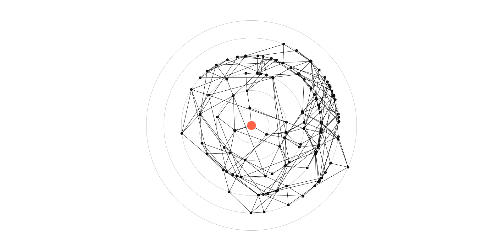
Bounding the extent with maxdist
Since the radius of a vertex equals its graph distance, a few remote vertices can dominate the frame. maxdist keeps the rings up to that distance intact and compresses everything beyond it onto a narrow band, keeping the angles:
layout = Egocentric(; focus, maxdist=4)
f, ax, p = graphplot(g; layout, node_color, node_size, edge_width=0.5)
for r in 1:4
    arc!(ax, Point2f(0), r, -pi, pi; color=(:gray, 0.5), linewidth=0.5)
end
hidedecorations!(ax); hidespines!(ax); ax.aspect = DataAspect(); f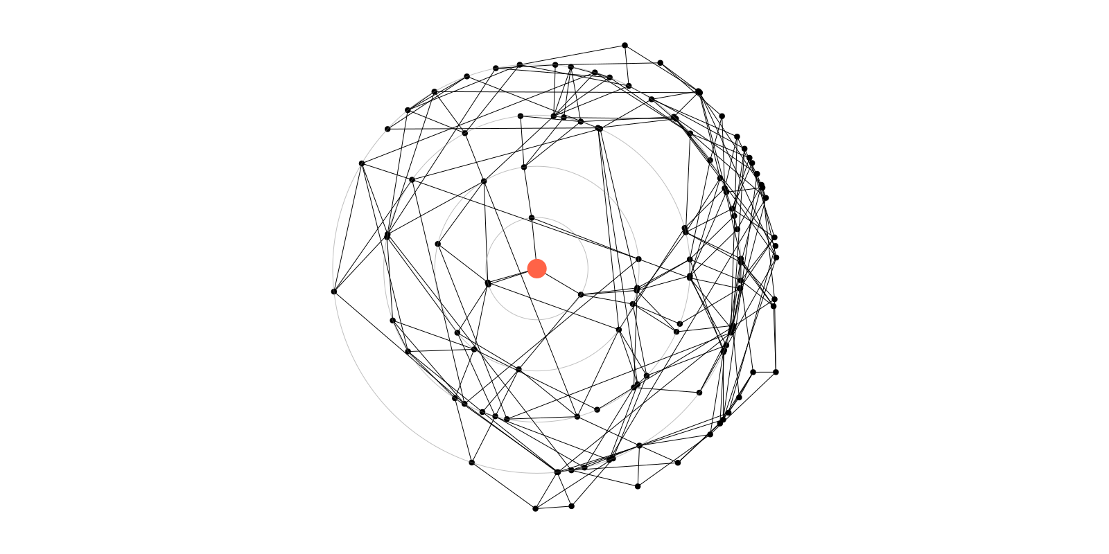
Passing a number instead of a function, e.g. compress=1, collapses everything past maxdist onto a single outer ring, which is a compact way to show "further away than maxdist" without saying how much further.
Iterator Example
layout = Egocentric(; focus)
f, ax, p = graphplot(g; layout, node_color, node_size, edge_width=0.5)
iterator = LayoutIterator(layout, g)
record(f, "egocentric_animation.mp4", iterator; framerate = 10) do pos
    p[:node_pos][] = pos
    autolimits!(ax)
endShell/Circular Layout
NetworkLayout.Shell — Type
Shell(; kwargs...)(adj_matrix)
shell(adj_matrix; kwargs...)
Position nodes in concentric circles. Without further arguments all nodes will be placed on a circle with radius 1.0. Specify placement of nodes using the nlist argument.
Takes adjacency matrix representation of a network and returns coordinates of the nodes.
Keyword Arguments
Ptype=Float64: Determines the output typePoint{2,Ptype}.nlist=Vector{Int}[]Vector of Vector of node indices. Tells the algorithm, which nodes to place on which shell from inner to outer. Nodes which are not present in this list will be place on additional outermost shell.
This function started as a copy from IainNZ's GraphLayout.jl
g = smallgraph(:petersen)
layout = Shell(nlist=[6:10,])
f, ax, p = graphplot(g, layout=layout)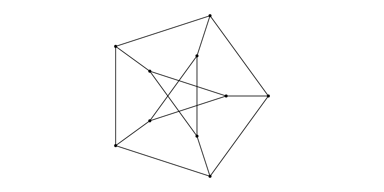
SquareGrid Layout
NetworkLayout.SquareGrid — Type
SquareGrid(; kwargs...)(adj_matrix)
squaregrid(adj_matrix; kwargs...)
Position nodes on a 2 dimensional rectagular grid. The nodes are placed in order from upper left to lower right. To skip positions see skip argument.
Takes adjacency matrix representation of a network and returns coordinates of the nodes.
Keyword Arguments
Ptype=Float64: Determines the output typePoint{2,Ptype}cols=:auto: Columns of the grid, the rows are determined automatic. If:autothe layout will be square-ish.dx=Ptype(1), dy=Ptype(-1): Ofsets between rows/cols.skip=Tuple{Int,Int}[]: Specify positions to skip when placing nodes.skip=[(i,j)]means to keep the position in thei-th row andj-th column empty.
g = Grid((12,4))
layout = SquareGrid(cols=12)
f, ax, p = graphplot(g, layout=layout, nlabels=repr.(1:nv(g)), nlabels_textsize=10, nlabels_distance=5)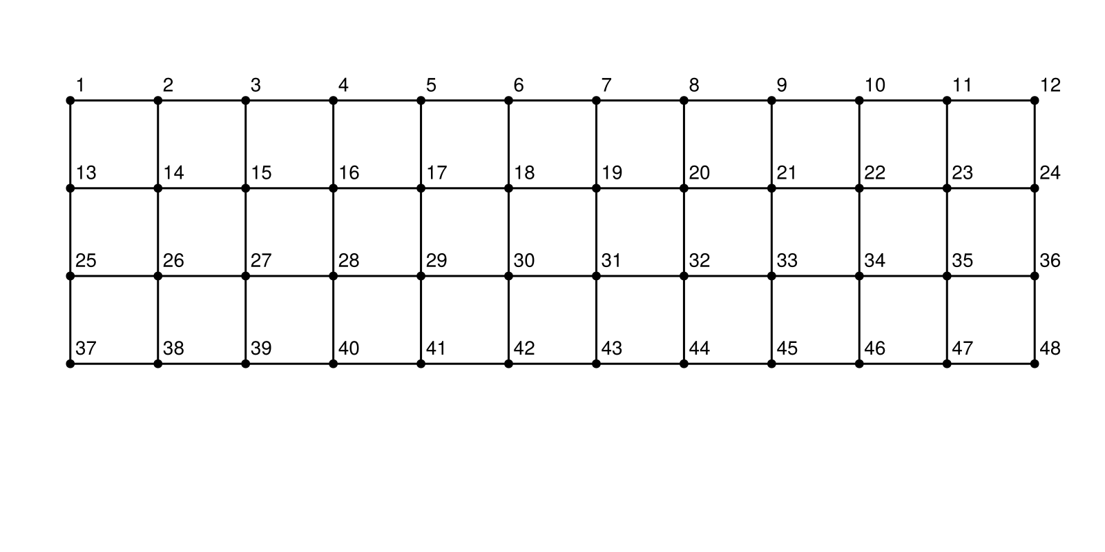
Spectral Layout
NetworkLayout.Spectral — Type
Spectral(; kwargs...)(adj_matrix)
spectral(adj_matrix; kwargs...)
This algorithm uses the technique of Spectral Graph Drawing. For reference see Koren (2003, doi 10.1007/3-540-45071-8_50).
Takes adjacency matrix representation of a network and returns coordinates of the nodes.
Keyword Arguments
dim=3,Ptype=Float64: Determines dimension and output typePoint{dim,Ptype}.nodeweights=Float64[]: Vector of weights. If network size does not match the length ofnodesizeuseonesinstead.
g = watts_strogatz(1000, 5, 0.03; seed=5)
layout = Spectral(dim=2)
f, ax, p = graphplot(g, layout=layout, node_size=0.0, edge_width=1.0)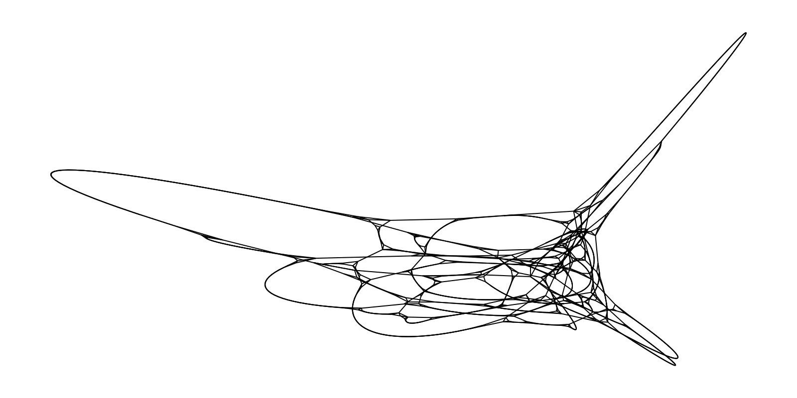
layout = Spectral()
f, ax, p = graphplot(g, layout=layout, node_size=0.0, edge_width=1.0)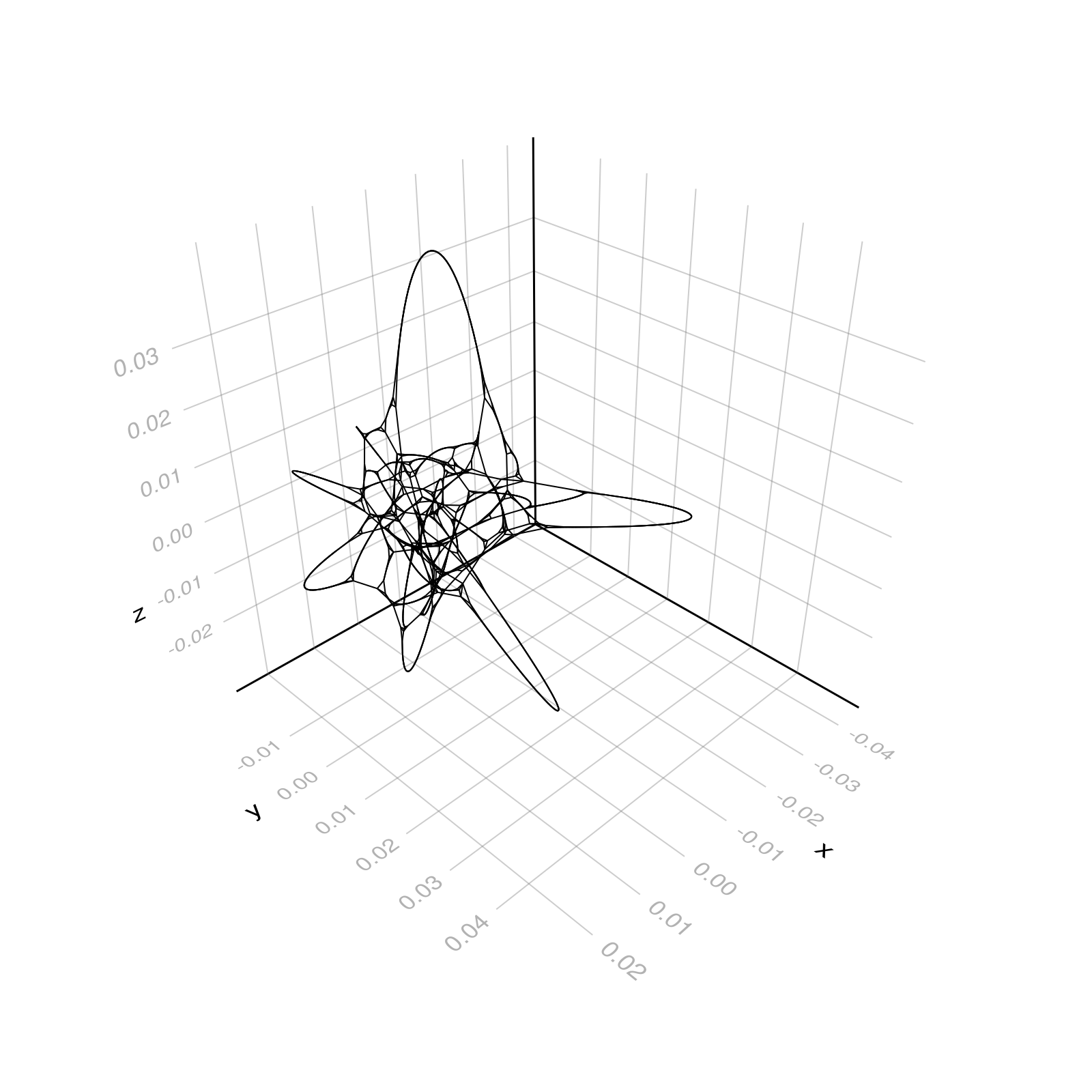
pin Positions in Interative Layouts
Sometimes it is desired to fix the positions of a few nodes while arranging the rest "naturally" around them. The iterative layouts Stress, Spring, SFDP and Egocentric allow to pin nodes to certain positions, i.e. those nodes will stay fixed during the iteration.
g = SimpleGraph(vcat(hcat(zeros(4,4), ones(4,4)), hcat(ones(4,4), zeros(4,4))))The keyword argument pin takes a Vector or a Dict of key - value pairs. The key has to be the index of the node. The value can take three forms:
idx => Point2(x,y)oridx => (x,y)overwrites the initial position of that vertex and pins it there,idx => true/falsepins or unpins the vertex, position is taken frominitialpos-keyword argument or random,idx => (false, true)allows for fine control over which coordinate to pin.
initialpos = Dict(1=>Point2f(-1,0.5),
                  3=>Point2f(1,0),
                  4=>Point2f(1,0))
pin = Dict(1=>true,
           2=>(-1,-0.5),
           3=>(true, false),
           4=>(true, false))
Example animation on how those keyword arguments effect different iterative layouts:
springl = Spring(;initialpos, pin, seed=2)
sfdpl   = SFDP(;initialpos, pin, tol=0.0)
stressl = Stress(;initialpos, pin, reltols=0.0, abstolx=0.0, iterations=100)

f = Figure(size=(1200,500))
ax1 = f[1,1] = Axis(f; title="Spring")
ax2 = f[1,2] = Axis(f; title="SFDP")
ax3 = f[1,3] = Axis(f; title="Stress")

for ax in [ax1, ax2, ax3]
    xlims!(ax,-2,2); ylims!(ax,-1.4,1.4); vlines!(ax, 1; color=:red); hidespines!(ax); hidedecorations!(ax)
end

node_color = vcat(:green, :green, :red, :red, [:black for _ in 1:4])
node_size = vcat([40 for _ in 1:4], [20 for _ in 1:4])
nlabels = vcat("1", "2", "3", "4", ["" for _ in 1:4])
nlabels_align = (:center, :center)
nlabels_color = :white
p1 = graphplot!(ax1, g; layout=springl, node_color, node_size, nlabels, nlabels_align, nlabels_color)
p2 = graphplot!(ax2, g; layout=sfdpl, node_color, node_size, nlabels, nlabels_align, nlabels_color)
p3 = graphplot!(ax3, g; layout=stressl, node_color, node_size, nlabels, nlabels_align, nlabels_color)

iterators = [LayoutIterator(l, g) for l in (springl, sfdpl, stressl)]
record(f, "pin_animation.mp4", zip(iterators...); framerate = 10) do (pos1, pos2, pos3)
    p1[:node_pos][] = pos1
    p2[:node_pos][] = pos2
    p3[:node_pos][] = pos3
end